The Moving City - Visualizing Public Transport
2020-05-09
This post was originally published on June 13, 2017 on Medium. I since migrated off from their platform and I'm republishing all of my old posts here.
This is a technical write-up on how hvv.live came to be, how the basic visualization is implemented and what nifty optimization we used to accomplish a satisfying user experience. If you haven’t checked out the map, head over to https://hvv.live and have a quick look. This will give you an impression on what we are going to talk about.
The Map
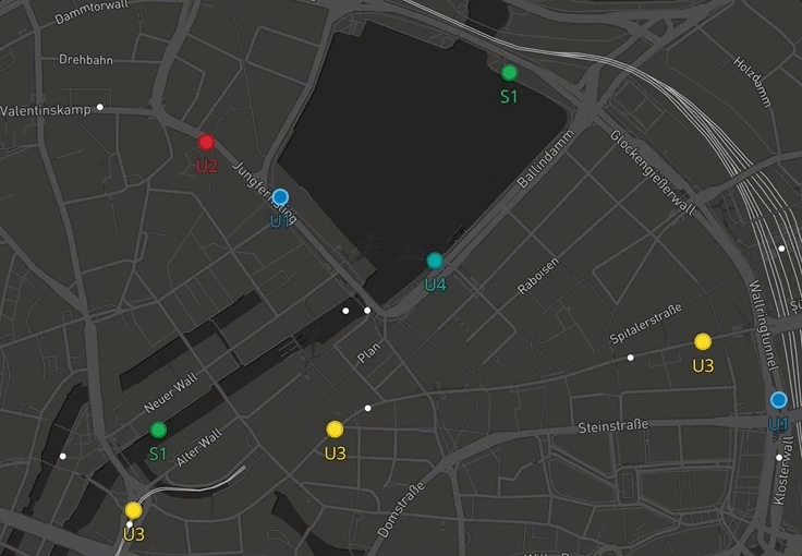
Just to get you up to speed on what the map shows:
- More or less real-time positions of all types of public transportation
- Depending on the filter setting you can see: Busses, (suburban) trains, subways & ships
- If you click on a moving vehicle, its complete route through the city is displayed (if available). Additional information about its next stop and current delay is given.
As the keen observer might have guessed, mapbox-gl-js forms the heart of the application. Everything you see on the map, from the circles with their labels to the colorful routes, is rendered directly by the map. Mapbox powerful data-driven styling features enable us to easily derive the appearance of a given vehicle from attached meta information like route number, vehicle type and current delay.
The Basics
What’s the magic that makes the circles move?
It’s no magic at all, it’s simple linear interpolation. But before we get to that, we need to figure out what our data looks like.
When the site is loaded, it will request the current tracks from the server. A track consists of a bunch of meta information and, more importantly, a geographical line geometry; it roughly translates to the route a vehicle drives between two way stations. The line is transmitted as a GeoJSON LineString , which is just a collection of longitude-latitude coordinate pairs: What you can see above as well is that each track contains a timestamp of its start and end time. This information is vital in order for us to determine the current position of the vehicle on the track. Here is what we do:
We need to figure out how far the vehicle has progressed on the line geometry we received. In order to figure out this progress we compare the start and end times with the current time:
progress = (now — start) / (end — start)
Our denominator is the full time span of the track, the numerator (the top part of the fraction) is the time span the vehicle has already driven. Now that we have a unitless indication of the vehicle’s progress on the track, we can transfer this on our line geometry.
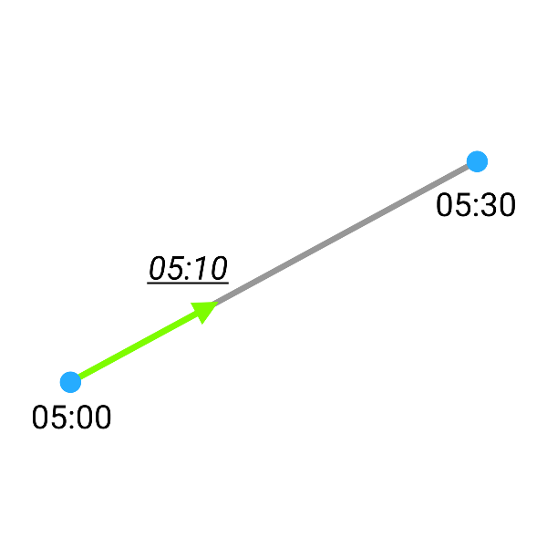
The complete distance of the line is trivial to calculate. All we have to do now, is to take this distance, multiply it with the progress and we get the distance we need to move along the line to figure out where our vehicle currently is. Figure 1 is demonstrating this part of the calculation. The blue dots represent the start and end points of our line with their corresponding timestamps. With the current time (5:10) we use the above approach to get to the resulting position.
On an implementation level we use cheap-ruler to calculate the line distance and to interpolate the point along the line. As we need to do this calculation for every track on every animation frame (that’s 60 times a second), we opted for cheap-ruler instead of turf.along . This means sacrificing precision for performance, but the loss is marginal compared to the speed gain. Now to render the moving circles, we just call setData as fast as possible on the Mapbox geojson source, the map will handle the rest…or will it?
The Optimizations
We quickly realized, that if we want to animate a few hundred points (at peak times there are up to 1.200 points on the map and every point is rendered), mapbox-gl-js will melt our CPUs. We also do render each position twice, one time as the colored circle and a second time as a semi-transparent blurry circle, which acts as a shadow for the first one. The library flawlessly renders static geometry, you can throw 50.000 (non-moving) points in there and it won’t break a sweat. Animating geometry on the other hand will quickly heat up your average hardware. As we didn’t want to fork mapbox-gl-js again to make internal changes, we needed to figure out how to pass on as little work as possible to the actual rendering: Minimize the work happening on each frame, in order to give the map enough time to fully render.
There is quite a simple solution for that problem: reduce the number of tracks we need to process before handing them off to the map. For this we added two different checks:
- Does a given line geometry intersect with the current viewport?
- Does a interpolated position reside within the current viewport?
Check #1 is run before the interpolation happens, the check might be a bit more expensive to make, but it is still cheaper than actually interpolating the position.
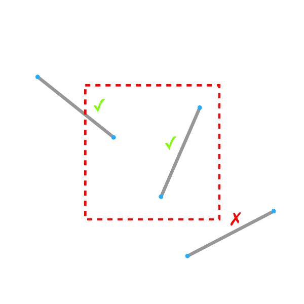
The diagram demonstrates what’s happening: If a line lays either partly or completely inside of the current viewport (the dashed red box) we need to hand it off to interpolation. If on the other hand it is fully outside of the viewport, we can just skip that line. To easily check if the line collides with the current viewport, all the track lines are stored in a spatial index. This allows us to quickly query which lines are relevant and which aren’t. We are using rbush which uses a R-tree data structure to store & retrieve spatial information.
Check #2 is run after we preprocessed the lines and generated the actual points. It’s a simple bounding box check.
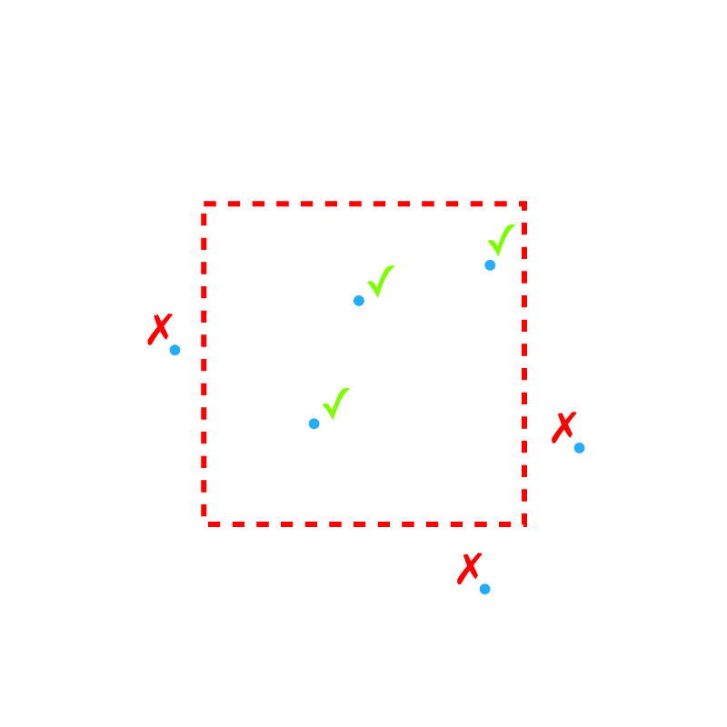
We just compare the longitude and latitude values of two diagonally opposite corners of our bounding box with the coordinates of a given point.
As a result of the two checks we receive the minimal set of points we need to render, with the help of aforemetioned high performances libraries we keep the preprocessing time below 2ms on an iPhone 7. This gives the map more than 14ms to render, which most of the time is enough. From our research the bottleneck isn’t really the GPU you use, but the number of CPU cores and their clock speed. As far as I know, mapbox-gl-js will convert any GeoJSON data to vector tiles before rendering that it. This conversion step is CPU-bound.
Another optimization we employed is not targeting rendering performance, but network traffic. If you click on a single vehicle, the complete route of that vehicle is fetched from the server. This again is a huge line geometry, containing a lot of single points. Early on we just sent a complete GeoJSON file to the client; depending on the route this can be up to 500kb of traffic (for a single click). Like every JSON GeoJSON does contain a lot of bloating characters…brackets and quotes. We don’t really need them to get the relevant information to the client: The point coordinates. That’s why we switched to just sending a simple CSV to the client; each line containing a coordinate pair. On the client we can efficiently reconstruct a valid GeoJSON object from those values. On average this halves the amount of data which needs to be transmitted.
The Future
Currently the application is pretty lean, it mostly does one thing: Animating a bunch of points on a map. But I’m proud that it is does this task very well. We are constantly looking into new ways to further improve that aspect, most recently we checked out deck.gl which uses Mapbox as a base map, but does its rendering in a separate context. The amount of data it is able to visualize is insane, deck.gl easily renders millions of data points; also animating a lot of points doesn’t seem to be an issue.
Of course we are considering to add more useful data to the map, which would make it an actually valuable application, e.g. highlighting vehicles and their stops in your current vicinity, delay notification and schedules…the possibilities are endless.
hvv.live was developed as a research project at Ubilabs and in my free time. I would be happy to answer questions or take any kind of advice.